Explore the generation and maintenance of membrane potential.
1. Introduction
This post serves as a comprehensive test of the Quarto deployment pipeline . We will verify: 1. \(\LaTeX\) RenderingPython Execution : Running simulation code during build time. 3. Visualization : Embedding generated figures. 4. Layout : Using callouts and columns.
2. Mathematical Model
The Leaky Integrate-and-Fire (LIF) neuron describes the evolution of membrane potential \(V(t)\) over time. The subthreshold dynamics are governed by the linear differential equation:
\[
\tau_m \frac{dV(t)}{dt} = -[V(t) - E_L] + R_m I_e(t)
\]
Where:
\(\tau_m\) : Membrane time constant (\(R_m C_m\) )\(E_L\) : Resting potential (Leak reversal potential)\(R_m\) : Membrane resistance\(I_e(t)\) : Input current
When \(V(t)\) reaches the threshold \(V_{th}\) , the neuron fires a spike, and \(V(t)\) is instantly reset to \(V_{reset}\) .
3. Simulation Code
Here we implement the Euler method to solve the equation numerically. The time step is \(\Delta t\) .
\[
V[t+1] = V[t] + \frac{\Delta t}{\tau_m} (- (V[t] - E_L) + R_m I_e)
\]
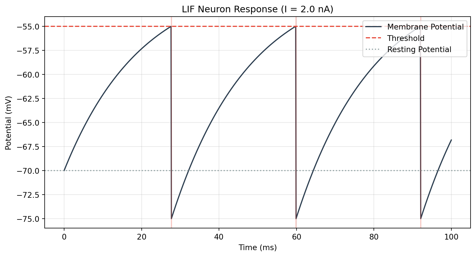
Code
import numpy as npimport matplotlib.pyplot as plt# 1. Parameters = 100.0 # Total time (ms) = 0.1 # Time step (ms) = np.arange(0 , T+ dt, dt)= 20.0 # Time constant (ms) = - 70.0 # Resting potential (mV) = 10.0 # Resistance (Mohm) = - 55.0 # Threshold (mV) = - 75.0 # Reset potential (mV) = 2.0 # Input current (nA) # 2. Initialization = np.zeros(len (time))0 ] = E_L= []# 3. Simulation Loop (Euler Method) for i in range (len (time)- 1 ):# Differential equation = (- (V[i] - E_L) + R_m * I_e) / tau_m+ 1 ] = V[i] + dV * dt# Spike mechanism if V[i+ 1 ] >= V_th:+ 1 ] = V_reset+ 1 ])# 4. Plotting = (10 , 5 ))= 'Membrane Potential' , color= '#2c3e50' , linewidth= 1.5 )= '#e74c3c' , linestyle= '--' , label= 'Threshold' )= '#95a5a6' , linestyle= ':' , label= 'Resting Potential' )# Mark spikes for t_spike in spikes:= '#e74c3c' , alpha= 0.3 )f"LIF Neuron Response (I = { I_e} nA)" )"Time (ms)" )"Potential (mV)" )= 'upper right' )True , alpha= 0.3 )# This confirms Python generated the plot
4. System Info
To ensure we are using the correct environment, here is the system information:
Code
import sysimport datetimeprint (f"Python Version: { sys. version. split()[0 ]} " )print (f"Build Date: { datetime. datetime. now(). strftime('%Y-%m- %d %H:%M:%S' )} " )
Python Version: 3.11.11
Build Date: 2026-01-26 17:41:38
5. Conclusion
If you can see the math equations properly rendered and the blue plot above, congratulations! Your Neuro-Engineering Blog stack is fully operational.
Next step: Integrate interactive Streamlit or Gradio modules via Docker.